Correcting for Periodicity Effects

Now that we have simulated our protein, we should run some analysis on the system. What types of data are important? This is an important question to ask before running the simulation, so you should have some ideas about the types of data you will want to collect in your own systems. For this tutorial, a few basic tools will be introduced.

The first is trjconv, which is used as a post-processing tool to strip out coordinates, correct for periodicity, or manually alter the trajectory (time units, frame frequency, etc). For this exercise, we will use trjconv to account for any periodicity in the system. The protein will diffuse through the unit cell, and may appear "broken" or may "jump" across to the other side of the box. To account for such behaviors, issue the following:

gmx trjconv -s md_0_10.tpr -f md_0_10.xtc -o md_0_10_noPBC.xtc -pbc mol -center

Select 1 ("Protein") as the group to be centered and 0 ("System") for output. We will conduct all our analyses on this "corrected" (more formally, "reimaged") trajectory.

Root-Mean-Square Deviation

Let's look at structural deviations first. GROMACS has a built-in utility for RMSD calculations called rms. To use rms, issue this command:

gmx rms -s md_0_10.tpr -f md_0_10_noPBC.xtc -o rmsd.xvg -tu ns

Choose 4 ("Backbone") for both the least-squares fit and the group for RMSD calculation. The -tu flag will output the results in terms of ns, even though the frames in the trajectory were written with time stamps in ps. This is done for clarity of the output (especially if you have a long simulation - "1e+05 ps" does not look as nice as "100 ns"). The output plot will show the RMSD relative to the structure present in the minimized, equilibrated system:

If we wish to calculate RMSD relative to the crystal structure, we could issue the following gmx rms command. Recall that the coordinates stored in em.tpr are the un-minimized, solvated system, so the protein coordinates are those taken directly from the 1AKI PDB entry, with added hydrogen atoms (which are not used for the RMSD calculation, anyway).

gmx rms -s em.tpr -f md_0_10_noPBC.xtc -o rmsd_xtal.xvg -tu ns

Plotted together, results look something like: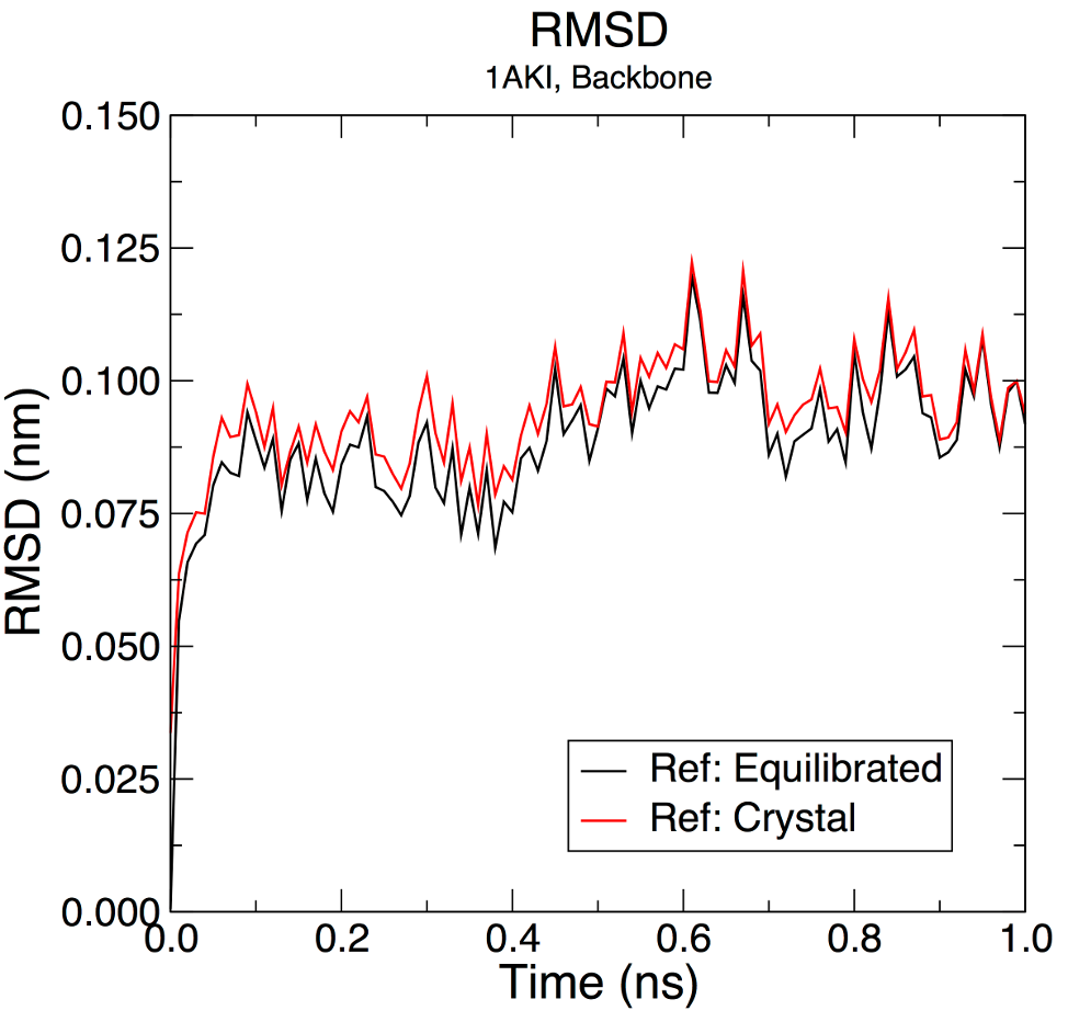

The raw data (gray and pink points) have been smoothed over a 500-ps (50-frame) window using the "Running Averages" feature in XmGrace (solid lines). This option is invoked by selecting Data -> Transformations -> Running Averages, then selecting the data set(s) to generate the smoothed windows, and the window length.

Both time series show the RMSD fluctuates around an average of 0.09 ± 0.01 nm (0.9 Å), indicating that the structure does not change very much. Subtle differences between the plots indicate that the structure at t = 0 ns is slightly different from this crystal structure. This is to be expected, since it has been energy-minimized, and because the position restraints are not 100% perfect, as discussed previously. Note that RMSD cannot be used as a metric to assess convergence of the simulation or determine "stability" of a system because it is a degenerate metric of structural change, and it is an extrinsic quantity. A large protein complex may have a 1.0-nm RMSD (10x higher than our result here) but be fairly invariant; the quantity is simply an accumulation of potentially very small deviations.