EM ensured that we have a reasonable starting structure, in terms of geometry and solvent orientation. To begin real dynamics, we must equilibrate the solvent and ions around the protein. If we were to attempt unrestrained dynamics at this point, the system may collapse. The reason is that the solvent is mostly optimized within itself, and not necessarily with the solute. It needs to be brought to the temperature we wish to simulate and establish the proper orientation about the solute (the protein). After we arrive at the correct temperature (based on kinetic energies), we will apply pressure to the system until it reaches the proper density.

Remember that posre.itp file that pdb2gmx generated a long time ago? We're going to use it now. The purpose of posre.itp is to apply a position restraining force on the heavy atoms of the protein (anything that is not a hydrogen). Movement is permitted, but only after overcoming a substantial energy penalty. The utility of position restraints is that they allow us to equilibrate our solvent around our protein, without the added variable of structural changes in the protein. The origin of the position restraints (the coordinates at which the restraint potential is zero) is provided via a coordinate file passed to the -r option of grompp.

Equilibration is often conducted in two phases. The first phase is conducted under an NVT ensemble (constant Number of particles, Volume, and Temperature). This ensemble is also referred to as "isothermal-isochoric" or "canonical." The timeframe for such a procedure is dependent upon the contents of the system, but in NVT, the temperature of the system should reach a plateau at the desired value. If the temperature has not yet stabilized, additional time will be required. Typically, 50-100 ps should suffice, and we will conduct a 100-ps NVT equilibration for this exercise. Depending on your machine, this may take a while (just under an hour if run in parallel on 16 cores or so). Get the .mdp file here.

We will call grompp and mdrun just as we did at the EM step:

gmx grompp -f nvt.mdp -c em.gro -r em.gro -p topol.top -o nvt.tpr

gmx mdrun -deffnm nvt

A full explanation of the parameters used can be found in the GROMACS manual, in addition to the comments provided. Take note of a few parameters in the .mdp file:

• gen_vel = yes: Initiates velocity generation. Using different random seeds (gen_seed) gives different initial velocities, and thus multiple (different) simulations can be conducted from the same starting structure.
• tcoupl = V-rescale: The velocity rescaling thermostat is an improvement upon the Berendsen weak coupling method, which did not reproduce a correct kinetic ensemble.
• pcoupl = no: Pressure coupling is not applied.

Let's analyze the temperature progression, again using energy:

gmx energy -f nvt.edr -o temperature.xvg

Type "16 0" at the prompt to select the temperature of the system and exit. The resulting plot should look something like the following: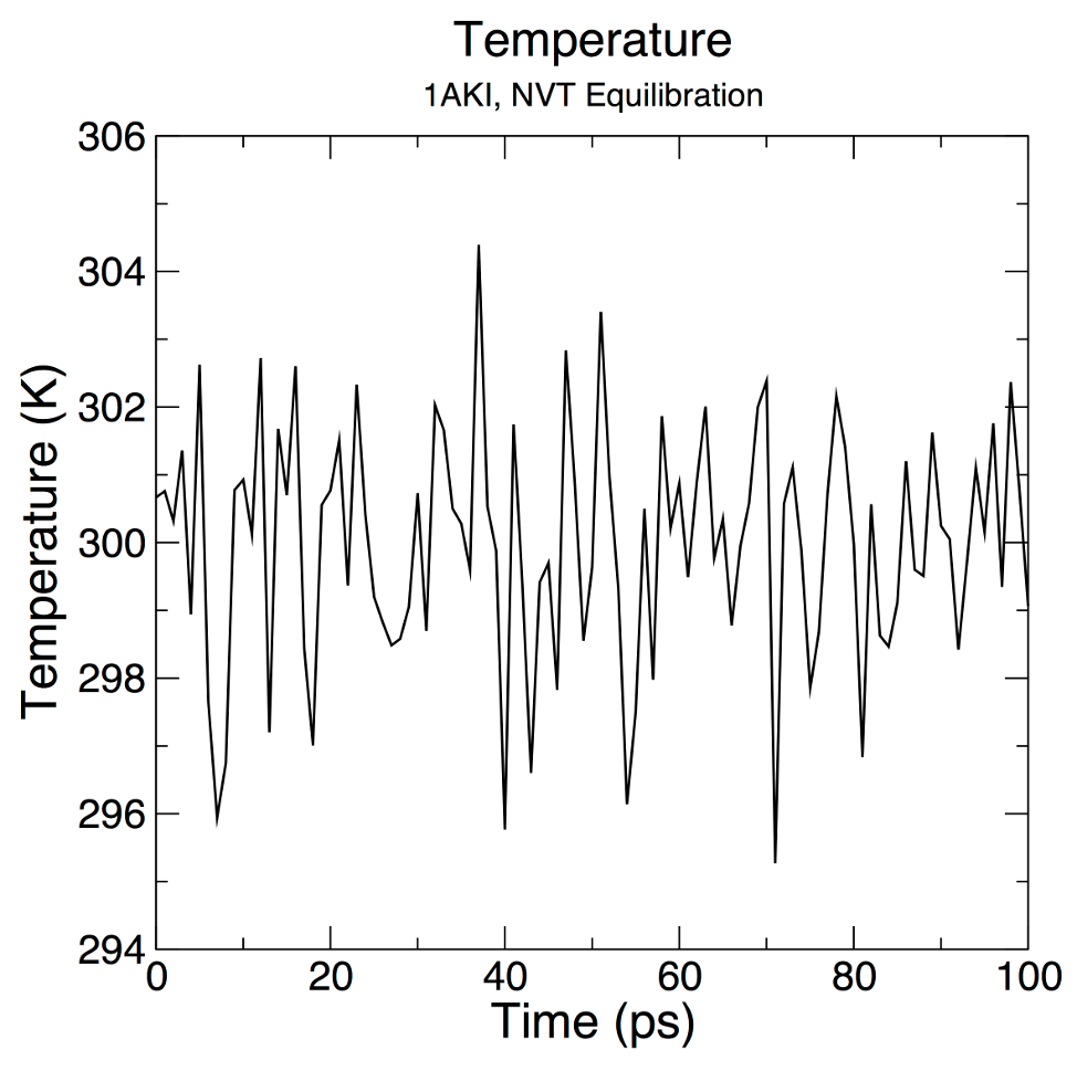

From the plot, it is clear that the temperature of the system quickly reaches the target value (300 K), and remains stable over the remainder of the equilibration. For this system, a shorter equilibration period (on the order of 50 ps) may have been adequate.