One common application of calculating free energies is to determine the of ΔG of binding between a ligand and a receptor (e.g., a protein), you would need to perform (de)coupling of the ligand in complex with the receptor and in bulk solution, since ΔG is (in this case) the sum of the free energy change of complexation of the ligand and receptor (i.e. the introduction of the ligand into the binding site) and the free energy of desolvating the ligand (i.e. removing it from solution):

ΔG of binding will be the difference between these two states, and can be calculated through the use of the following (somewhat simplified) thermodynamic cycle, wherein ΔG₁ is ΔG_solvation and ΔG₃ is ΔG_complexation in the equations above.

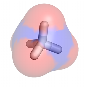
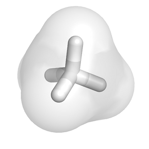
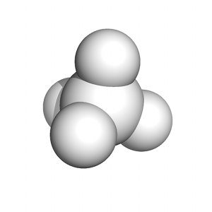
A particularly detailed thermodynamic cycle for this type of process can be found in Figure 1 of this paper.

The transformation of a fully-interacting species (e.g., the ligand) into a "dummy" (a set of atomic centers in the configuration of the ligand that does not engage in any nonbonded interactions with its surroundings) requires turning off both van der Waals interactions (as demonstrated in this tutorial) and Coulombic interactions between the solute of interest and its surrounding environment. The complete series of transformations for methane is shown below:

Fully-interacting	No charges, full LJ	Dummy molecule

In the above thermodynamic cycle, ΔG₁ and ΔG₃ actually represent the introduction of the ligand (starting as a dummy molecule), i.e. coupling rather than decoupling. The thermodynamic cycle above is extremely basic, and does not account for considerations like orientational restraints, conformational changes of the protein, etc. None of this literature will be discussed here. For most small molecules (generically named "LIG" below), the following settings might seem attractive:

     couple-moltype    = LIG
     couple-intramol   = no
     couple-lambda0    = none
     couple-lambda1    = vdw-q 

Special care must be taken in this case. In previous versions of GROMACS, such an approach was likely to be very unstable because removal of van der Waals terms while a system retains some charge allows oppositely-charged atoms to interact very closely (in the absence of the full effects of an electron cloud). The result would be unstable configurations and unreliable energies, even if the systems didn't collapse. Thus, it is more sound to approach the (de)coupling sequentially. In version 5.0, this is very easily done with the new λ vector capabilities:

    couple-moltype          = LIG
    couple-intramol         = no
    couple-lambda0          = none
    couple-lambda1          = vdw-q
    init_lambda_state       = 0
    calc_lambda_neighbors   = 1
    vdw_lambdas             = 0.00 0.05 0.10 ... 1.00 1.00 1.00 ... 1.00
    coul_lambdas            = 0.00 0.00 0.00 ... 0.00 0.05 0.10 ... 1.00

In this case, the λ value for Coulombic interactions is always zero while the λ value for transforming van der Waals interactions changes. Then, the van der Waals interactions are fully on (λ = 1.00) while the Coulombic interactions are gradually turned on. Keeping track of the states to which λ = 0 and λ = 1 correspond is key to this process. In the above case, couple-lambda0 says interactions are off, while couple-lambda1 means interactions are on.

These types of transformations can be useful for calculating hydration/solvation free energies, since this quantity is often used as target data in force field parametrization.