GROMACS Tutorial
Step Seven: Analysis
|
The bar module of GROMACS makes the calculation of ΔGAB very simple. Simply collect all of the md*.xvg files that were produced by mdrun (one for each value of λ) in the working directory and run gmx bar: gmx bar -f md*.xvg -o -oi The program will print lots of useful information to the screen, in addition to producing three output files: bar.xvg, barint.xvg, and histogram.xvg. The screen output from gmx bar should look something like:
Detailed results in kT (see help for explanation):

 lam_A  lam_B      DG   +/-     s_A   +/-     s_B   +/-   stdev   +/-
     0      1    0.08  0.00    0.03  0.00    0.03  0.00    0.25  0.00
     1      2    0.07  0.00    0.03  0.00    0.03  0.00    0.25  0.00
     2      3    0.06  0.00    0.03  0.00    0.04  0.00    0.26  0.00
     3      4    0.04  0.00    0.04  0.00    0.05  0.00    0.28  0.00
     4      5    0.02  0.00    0.03  0.00    0.04  0.00    0.29  0.00
     5      6    0.00  0.00    0.05  0.00    0.06  0.00    0.30  0.00
     6      7   -0.02  0.00    0.05  0.00    0.06  0.00    0.32  0.00
     7      8   -0.06  0.01    0.06  0.00    0.07  0.00    0.35  0.01
     8      9   -0.09  0.01    0.06  0.00    0.07  0.00    0.37  0.00
     9     10   -0.14  0.01    0.08  0.00    0.10  0.01    0.41  0.01
    10     11   -0.22  0.01    0.09  0.01    0.12  0.01    0.46  0.00
    11     12   -0.31  0.01    0.12  0.01    0.15  0.01    0.51  0.01
    12     13   -0.45  0.01    0.17  0.01    0.20  0.01    0.57  0.00
    13     14   -0.59  0.01    0.16  0.02    0.17  0.02    0.58  0.01
    14     15   -0.62  0.01    0.11  0.01    0.11  0.01    0.47  0.00
    15     16   -0.54  0.01    0.06  0.01    0.06  0.01    0.35  0.00
    16     17   -0.42  0.00    0.03  0.01    0.03  0.01    0.25  0.00
    17     18   -0.28  0.00    0.02  0.00    0.02  0.00    0.18  0.00
    18     19   -0.16  0.00    0.01  0.00    0.01  0.00    0.13  0.00
    19     20   -0.05  0.00    0.00  0.00    0.00  0.00    0.10  0.00

Final results in kJ/mol:

point      0 -      1,   DG  0.19 +/-  0.00
point      1 -      2,   DG  0.17 +/-  0.01
point      2 -      3,   DG  0.14 +/-  0.00
point      3 -      4,   DG  0.09 +/-  0.01
point      4 -      5,   DG  0.06 +/-  0.00
point      5 -      6,   DG  0.01 +/-  0.01
point      6 -      7,   DG -0.06 +/-  0.01
point      7 -      8,   DG -0.14 +/-  0.02
point      8 -      9,   DG -0.23 +/-  0.01
point      9 -     10,   DG -0.35 +/-  0.01
point     10 -     11,   DG -0.53 +/-  0.01
point     11 -     12,   DG -0.77 +/-  0.03
point     12 -     13,   DG -1.12 +/-  0.03
point     13 -     14,   DG -1.46 +/-  0.02
point     14 -     15,   DG -1.53 +/-  0.04
point     15 -     16,   DG -1.35 +/-  0.02
point     16 -     17,   DG -1.04 +/-  0.01
point     17 -     18,   DG -0.70 +/-  0.01
point     18 -     19,   DG -0.40 +/-  0.00
point     19 -     20,   DG -0.13 +/-  0.00

total      0 -     20,   DG -9.13 +/-  0.09
The value of ΔGAB I obtained is -9.13 ± 0.09 kJ mol-1, or -2.18 ± 0.02 kcal mol-1. Since the process I conducted for this demonstration was the decoupling of methane, the reverse process (the introduction of uncharged methane into water, thus the actual hydration energy of the process) corresponds to a ΔGAB of 2.18 ± 0.02 kcal mol-1 (assuming reversibility), in good agreement with the value obtained by Shirts et al. of 2.24 ± 0.01 kcal mol-1 (per Table II of the Supporting Information of that paper), despite the fact that I used about half the number of λ vectors for the van der Waals transformation than the original authors did, in addition to the other changes described previously. Technically, this is all we need to do to arrive at our answer, but gmx bar also prints a number of useful output files (all of which are optional). Their contents are worth exploring here, as they provide a great level of detail into the decoupling process and the success of sampling. Output file 1: bar.xvgLet's take a look at the other output files that gmx bar gave us, starting with bar.xvg. This output file plots the relative free energy differences for each interval of λ (i.e., between neighboring Hamiltonians), and should look something like this (after re-plotting as a bar graph rather than the default line representation, and adding a few grid lines for perspective): 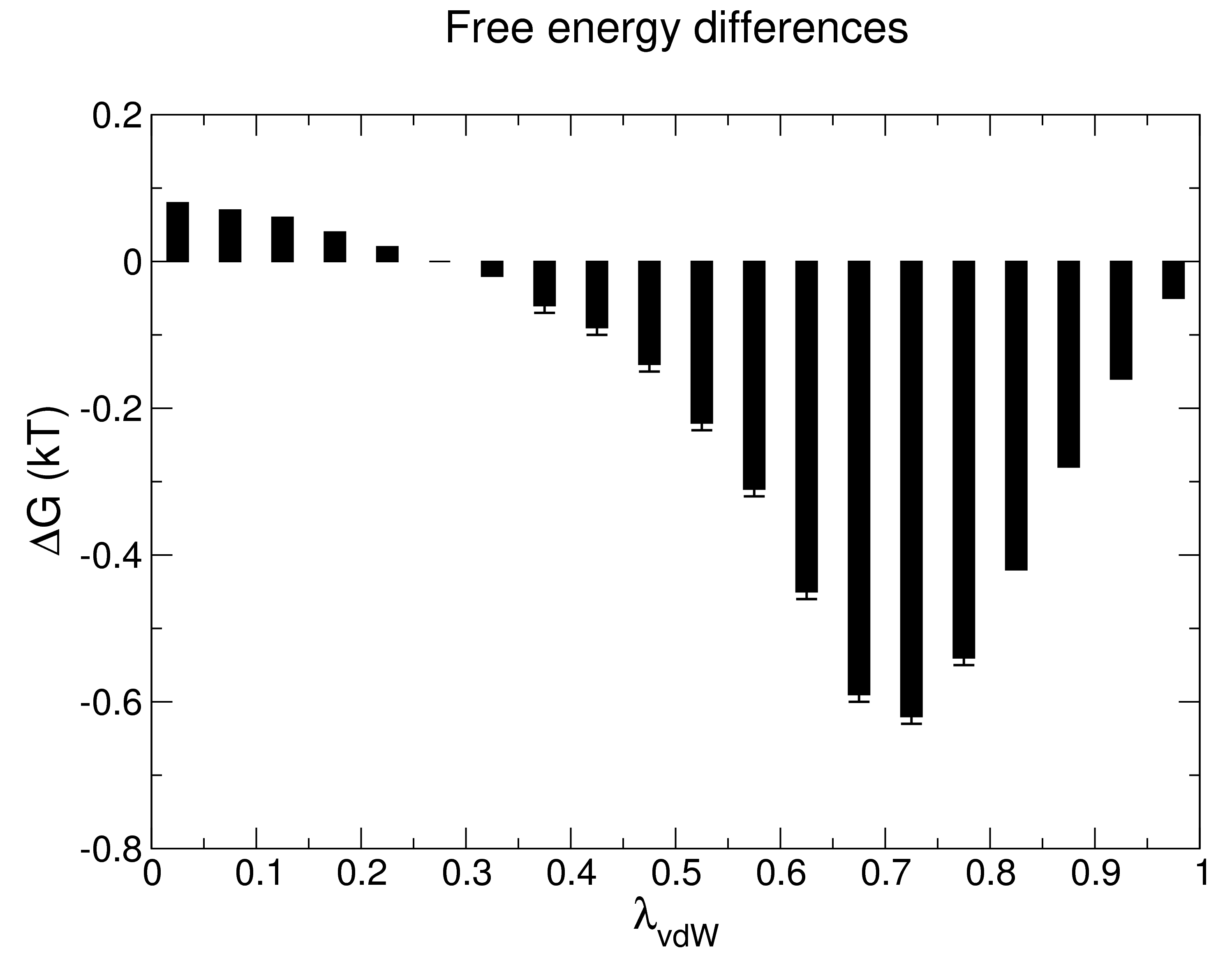
The vertical gray lines indicate the values of λ utilized in the decoupling process conducted here. Thus, each black bar indicates the free energy difference between neighboring values of λ. In bar.xvg, we get the first look at what calc_lambda_neighbors was doing during the simulations. For example, in our simulation of init_lambda_state = 0, the free energy at λ = 0.05 (the nearest neighboring window, as specified by calc_lambda_neighbors = 1) was evaluated every nstdhdl (10) steps. These "foreign" λ calculations result in energetic overlap between the values of λ, such that we have phase space overlap and adequate sampling. Interested readers should refer to the paper by Wu and Kofke cited in the gmx bar description for a discussion of this concept as well as the interpretation of the entropy values sA and sB. Thus, the free energy change from λ = 0 to λ = 1 is simply the sum of the free energy changes of each pair of neighboring λ simulations, which are plotted in bar.xvg. The values of ΔG correspond to the first half of the output printed to the screen by gmx bar. The second half of the screen output contains these same values of ΔG, converted to kJ mol-1 (1 kT = 2.478 kJ mol-1 at 298 K). Output file 2: barint.xvgThe barint.xvg file plots the cumulative ΔG as a function of λ. In barint.xvg, the point at λ = 1 corresponds to the sum of ΔG from λ vector 0 to λ vector 1, as indicated in the screen output above:
 lam_A  lam_B      DG   +/-     s_A   +/-     s_B   +/-   stdev   +/-
     0      1    0.08  0.00    0.03  0.00    0.03  0.00    0.25  0.00
     1      2    0.07  0.00    0.03  0.00    0.03  0.00    0.25  0.00
Therefore, the value of the cumulative ΔG in barint.xvg at λ = 0 is zero, and the value at λ = 0.1 is 0.0 + 0.08 = 0.08, and this is the value we find in barint.xvg. Below is the plot of barint.xvg (blue) alongside the contents of bar.xvg (black, the values of ΔG between λ values) to illustrate the cumulative ΔG. By taking the value of ΔG at λ = 20 (-3.69 kT), we can recover the value of ΔG shown above (-9.14 kJ mol-1). The difference between the value here (-9.14) and above (-9.13) is due to rounding error from using only two decimal places, whereas the bar program is using full precision in its calculations above, but printing only two decimal places for all output. 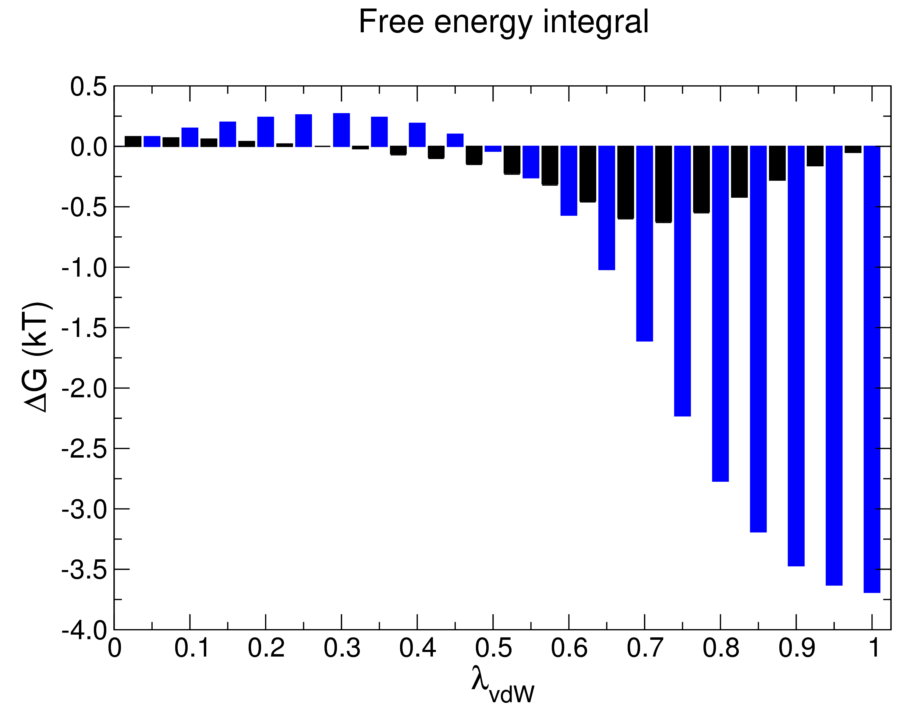
|
Site design and content copyright Justin Lemkul
Problems with the site? Send them to the Webmaster