To conduct umbrella sampling, one must generate a series of configurations along a reaction coordinate, ζ. Some of these configurations will serve as the starting configurations for the umbrella sampling windows, which are run in independent simulations. The figure below illustrates these principles. The top image illustrates the pulling simulation we will run now, conducted in order to generate a series of configurations along the reaction coordinate. These configurations are extracted after the simulation is complete (dashed arrows in between the top and middle images). The middle image corresponds to the independent simulations conducted within each sampling window, with the center of mass of the free peptide restrained in that window by an umbrella biasing potential. The bottom images shows the ideal result as a histogram of configurations, with neighboring windows overlapping such that a continuous energy function can later be derived from these simulations.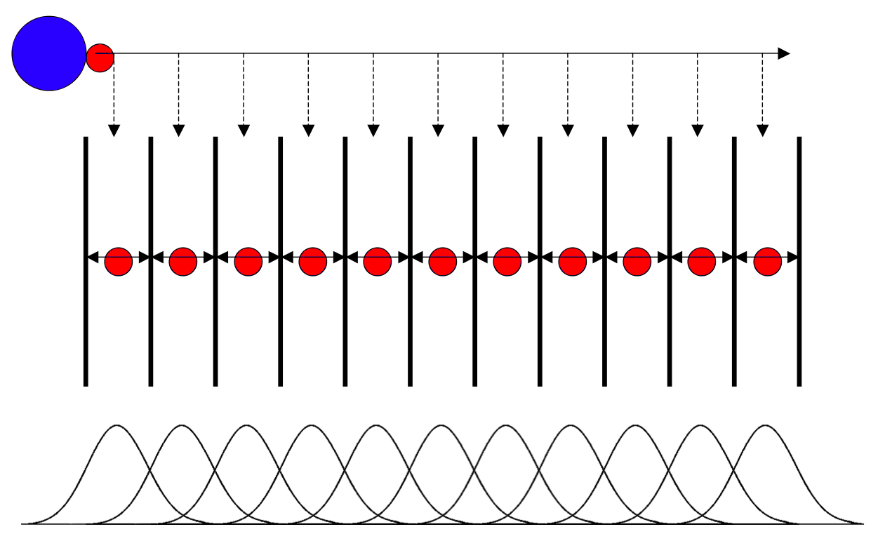

For this example, the reaction coordinate is the z-axis. To generate these configurations, we must pull peptide A away from the protofibril. We will pull over the course of 500 ps of MD, saving snapshots every 1 ps. This setup has been established based on trial-and-error to obtain a reasonable distribution of configurations. In other systems, it may be necessary to save configurations more often, or sufficient to save configurations less often. The idea is to capture enough configurations along the reaction coordinate to obtain regular spacing of the umbrella sampling windows, in terms of center-of-mass distance between peptides A and B.

The .mdp file for this pulling can be found here. A brief explanation of the pulling options used is as follows:

; Pull code
pull                    = yes
pull_ncoords            = 1         ; only one reaction coordinate
pull_ngroups            = 2         ; two groups defining one reaction coordinate
pull_group1_name        = Chain_A
pull_group2_name        = Chain_B
pull_coord1_type        = umbrella  ; harmonic potential
pull_coord1_geometry    = distance  ; simple distance increase
pull_coord1_dim         = N N Y     ; pull along z
pull_coord1_groups      = 1 2       ; groups 1 (Chain A) and 2 (Chain B) define the reaction coordinate
pull_coord1_start       = yes       ; define initial COM distance > 0
pull_coord1_rate        = 0.01      ; 0.01 nm per ps = 10 nm per ns
pull_coord1_k           = 1000      ; kJ mol^-1 nm^-2

• pull = yes: tells grompp to read settings for COM pulling. If omitted, all pull settings are ignored
• pull_ncoords = 1: defines the number of reaction coordinates that are present in the system. This setting allows for multiple biases to be set simultaneously for the purposes of multi-dimensional free energy calculations, but for our purposes here, only one reaction coordinate exists.
• pull_ngroups = 2: there are two groups that define the ends of the reaction coordinate. The reaction coordinate is the COM distance between these two groups.
• pull_group1_name = Chain_A and pull_group2_name = Chain_B: the names of the groups used by the pull code, which are read from the index file. Since there are two groups specified in this system (pull_ngroups = 2 on the previous line), then two names must be provided.
• pull_coord1_type = umbrella: using a harmonic potential to pull. IMPORTANT: This procedure is NOT umbrella sampling. The harmonic potential allows the force to vary according to the nature of the interactions of peptide A with peptide B. That is, the force will build up until certain critical interactions are broken. See our paper for details. For the purposes of generating the initial configurations for umbrella sampling, you can actually use different combinations of pull settings (pull_coord1_type and pull_coord1_geometry), but when it comes time for the actual umbrella sampling (in the next step) you MUST be using pull_coord1_type = umbrella. It is very important that you do not apply extremely fast pulling rates or extremely strong force constants, which can seriously deform elements of your system. Please refer to paper (particularly the Supporting Information) for how we chose to validate the pull rate used. Also note that this is the first setting in which "coord1" appears as part of the keyword name. For every reaction coordinate defined (pull_ncoords), all of the settings shown above are necessary. If there is a second reaction coordinate, the settings would be named "coord2," a third "coord3," and so on.
• pull_coord1_geometry = distance: see the note the in .mdp file; you can also use position, direction, or direction-periodic, but changes will have to be made to other pulling parameters. Doing so is left as an exercise to the user.
• pull_coord1_dim = N N Y: we are applying a bias only in the z-dimension. Thus, x and y are set to "no" (N) and z is set to "yes" (Y).
• pull_coord1_groups: the reaction coordinate connects groups 1 and 2.
• pull_coord1_start = yes: the initial COM distance is the reference distance for the first frame. More on this setting in the next phase, during which actual umbrella sampling simulations are carried out
• pull_coord1_rate = 0.01: the rate at which the imaginary spring attached to our pull groups is elongated. This type of pulling is also called "constant velocity" due to the fact that this rate is fixed.
• pull_coord1_k = 1000: the force constant on the spring used for pulling.

Remember that #ifdef POSRES_B statement we added to topol_B.itp a while ago? We're going to use it now. By restraining peptide B of the protofibril, we are able to more easily pull peptide A away. Due to the extensive non-covalent interactions between chains A and B, if we did not restrain chain B, we would end up simply towing the whole complex along the simulation box, which wouldn't accomplish much.

We will need to define some custom index groups for this pulling simulation. Use make_ndx:

gmx make_ndx -f npt.gro
...
 > r 1-27
 > name 19 Chain_A
 > r 28-54
 > name 20 Chain_B
 > q

Now, run the steered MD simulation:

gmx grompp -f md_pull.mdp -c npt.gro -p topol.top -r npt.gro -n index.ndx -t npt.cpt -o pull.tpr
gmx mdrun -deffnm pull -pf pullf.xvg -px pullx.xvg

The process will play out something like the following:

There is no displacement for some time, as the force on the imaginary spring builds up until it is sufficient to overcome the restoring forces within the protofibril structure. About halfway through the SMD simulation, chain A begins to dissociate from chain B. This process is also visible in the force on the spring over time, stored in pullf.xvg: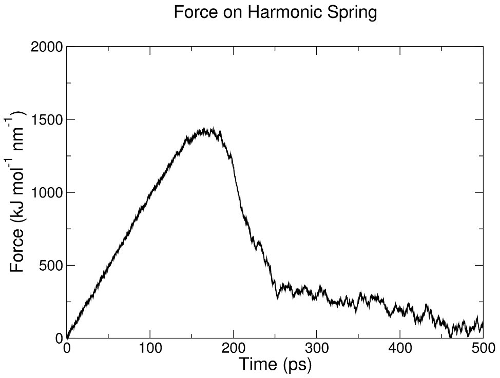

To prepare the individual umbrella sampling windows, we will need to extract useful frames from the SMD trajectory. The easiest way I have found to do this is the following:

1. Define the spacing of the windows (generally 0.1 - 0.2 nm)
2. Extract all the frames from the pulling trajectory that was just produced
3. Measure the COM distance of each of these frames between the two groups defining the reaction coordinate
4. Use the selected frames for umbrella sampling input

To extract the frames from your trajectory (traj.xtc), use trjconv (save the whole system, group 0, when prompted):

gmx trjconv -s pull.tpr -f pull.xtc -o conf.gro -sep

A series of coordinate files (conf0.gro, conf1.gro, etc) will be produced, corresponding to each of the frames saved in the continuous pulling simulation. To iteratively call gmx distance on all of these (501!) frames that were generated, I have written a Bash script that takes care of this task. It will print a file called "summary_distances.dat" that contains this information. The script can be found here.

Look at the contents of summary_distances.dat to see the progression of COM distance between chain A and chain B over time. Make note of the configurations to be used for umbrella sampling, based on the desired spacing. That is, if you want 0.2-nm spacing, you might find the following lines in summary_distances.dat:

6     0.500
...
160    0.704

You would then use conf6.gro and conf160.gro as the starting configurations of two adjacent umbrella sampling windows. Make note of all the configurations you wish to use before continuing. For the purposes of this tutorial, identifying configurations with 0.2-nm spacing will suffice, although in the original work a different spacing was used to more thoroughly define the free energy at the energy minimum.