|
The free energy change of transforming a system from state A to state B, ΔGAB, is a function of a coupling parameter, λ, which indicates the level of change that has taken place between states A and B, that is, the extent to which the Hamiltonian has been perturbed and the system has been transformed. Simulations conducted at different values of λ allow us to plot a ∂H/∂λ curve, from which ΔGAB is derived. The first step in planning free energy calculations is how many λ points will be used to describe the transformation from state A (λ = 0) to state B (λ = 1), with the goal of collecting adequate data to exhaustively sample phase space and produce a reliable ∂H/∂λ curve.
For decoupling Coulombic interactions, which depend linearly upon λ, an equidistant λ spacing from 0 to 1 should usually suffice, with λ spacing values of of 0.05-0.1 being common. Note that this is a broad generalization, and in fact many molecules will require a great deal more finesse, such as those that interact very strongly with the surrounding environment through hydrogen bonding. In this case, λ spacing may need to be decreased, such that more points are used, perhaps even in an asymmetric fashion.
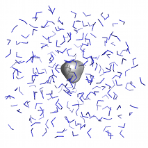
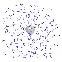
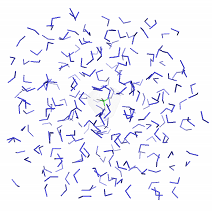
For decoupling van der Waals interactions, λ spacing can be much trickier. For reasons described by Shirts et al. and elsewhere, a great deal of λ points may be necessary to properly describe the transformation. Clustering λ points in regions where the slope of the ∂H/∂λ curve is steep may be necessary. For the purposes of this tutorial, we will use equidistant λ spacing of 0.05, but in many cases, one may need to use different spacing, especially clustering values in the range of 0.6 ≤ λ ≤ 0.8.
For each value of λ, a complete workflow (energy minimization, equilibration, and data collection) must be conducted. I generally find it most efficient to run these jobs as batches, passing the output of one step directly into the next. The workflow utilized here will be:
- Steepest descents minimization
- NVT equilibration
- NPT equilibration
- Data collection under an NPT ensemble
The .mdp files for the different steps of the tutorial (for λ = 0 only) are provided at the following links:
I am also making available an accessory Perl script, write_mdp.pl, that you can use to very quickly produce all of the input files needed for running these simulations. You can also download a shell script (job.sh) for running these jobs according to the workflow I will describe.
If you issue:
perl write_mdp.pl em_steep.mdp
You will receive files named em_steep_0.mdp, em_steep_1.mdp, ... em_steep_20.mdp, with the relevant values of init_lambda_state inserted into the filename. Analogously, you can produce the rest of your .mdp files in the same way (nvt.mdp, npt.mdp, and md.mdp).
In job.sh, you will need to change the values of $FREE_ENERGY and $MDP, otherwise the script certainly won't work.
Notes on .mdp settings
Before proceeding, it is important to understand the free energy-related settings in the .mdp files (using em_steep_0.mdp as an example). They are the same for all steps in the workflow. I will assume that you are familiar with the other settings found in the .mdp file. If this is not the case, please refer to some more basic tutorial material before proceeding.
|
|
free_energy = yes
|
Indicates that we are doing a free energy calculation, and that interpolation between the A and B states of the chosen molecule (defined below) will occur.
|
|
|
init_lambda_state = 0
|
In previous GROMACS versions, the "init_lambda" keyword specified a single value of λ directly. Since version 5.0, λ is now a vector that allows for transformation of bonded and nonbonded interactions. With the init_lambda_state keyword, we specify an index (starting from zero) of the vector to be utilized in the simulation (more on this later).
|
|
|
delta_lambda = 0
|
The value of λ can be incremented by some amount per timestep (i.e., δλ/δt) in a technique called "slow growth." This method can have significant errors associated with it, and thus we will make no time-dependent changes to our λ values.
|
|
|
fep_lambdas = (nothing)
|
You will note that this keyword is not specified. In previous GROMACS versions, the use of init_lambda and foreign_lambda controlled the value of λi and the additional values of λ for which energy differences would be evaluated for configurations at λi. This is no longer the case. One can explicitly set values of λ in the fep_lambdas keyword, but instead we allow the calc_lambda_neighbors keyword (see below) to automatically determine these additional values.
|
|
|
calc_lambda_neighbors = 1
|
The number of neighboring windows for which energy differences are computed with respect to λi. For instance, if init_lambda_state is set to 10, then energy differences with respect to λ states 9 and 11 are computed during the run with calc_lambda_neighbors = 1.
|
|
|
vdw_lambdas = ...
|
An array of λ values for the transformation of van der Waals interactions.
|
|
|
coul_lambdas = ...
|
An array of λ values for the transformation of Coulombic (electrostatic) interactions.
|
|
|
bonded_lambdas = ...
|
An array of λ values for the transformation of bonded interactions.
|
|
|
restraint_lambdas = ...
|
An array of λ values for the transformation of restraints.
|
|
|
mass_lambdas = ...
|
An array of λ values for the transformation of atomic masses; used if tranforming the chemical nature of the molecule.
|
|
|
temperature_lambdas = ...
|
An array of λ values for the transformation of temperatures; used only for simulated tempering.
|
|
|
sc-alpha = 0.5
|
The value of the α scaling factor used in the "soft-core" Lennard-Jones equation. See equations 4.124 - 4.126 in the GROMACS manual, section 4.5.1, for a complete description of this term, as well as the next three.
|
|
|
sc-coul = no
|
Transform Coulombic interactions linearly. This is the default behavior, but is written out for clarity.
|
|
|
sc-power = 1.0
|
The power for λ in the soft-core equation.
|
|
|
sc-sigma = 0.3
|
The value of σ assigned to any atom types that have C6 or C12 parameters equal to zero or σ < sc-sigma (typically H atoms). This value is used in the soft-core Lennard-Jones equation.
|
|
|
couple-moltype = Methane
|
The name of the [moleculetype] in that will have its topology interpolated from state A to state B. Note that the name given here must match a [moleculetype] name, and not the residue name. In some cases these may be the same, but I have maintained different names for the [moleculetype] and component residue for instructive purposes.
|
|
|
couple-lambda0 = vdw
|
The types of nonbonded interactions that are present in state A between the interpolated [moleculetype] and the remainder of the system. The value "vdw" indicates that only van der Waals terms are active between methane and water; there are no solute-solvent Coulombic interactions.
|
|
|
couple-lambda1 = none
|
The types of nonbonded interactions that are present in state B between the interpolated [moleculetype] and the remainder of the system. The value "none" indicates that both van der Waals and Coulombic interactions are off in state B. Relative to couple-lambda0, this indicates that only van der Waals terms have been turned off.
|
|
|
couple-intramol = no
|
Do not decouple intramolecular interactions. That is, the λ factor is applied to only solute-solvent nonbonded interactions and not solute-solute nonbonded interactions.
Setting "couple-intramol = yes" is useful for larger molecules that may have intramolecular interactions occuring at longer distance (e.g. peptides or other polymers). Otherwise, distal parts of the molecule will interact via explicit pair interactions in an unnaturally strong manner (since solute-solvent interactions are weakened as a function of λ, but the intramolecular terms would not be), giving rise to configurations that will incorrectly bias the resulting free energy.
|
|
|
nstdhdl = 10
|
The frequency with which ∂H/∂λ and ΔH are written to dhdl.xvg. A value of 100 would probably suffice, since the resulting values will be highly correlated and the files will get very large. You may wish to increase this value to 100 for your own work.
|
|
There are also several differences in the .mdp settings that will be used here relative to the settings used by Shirts et al.:
- rlist=rcoulomb=rvdw=1.2. In order to use PME, rlist must be equal to rcoulomb, a check that was enforced in grompp sometime after the release of version 3.3.1. The Verlet cutoff scheme introduced in version 4.6 that allows for buffered neighbor lists also requires rvdw=rcoulomb. The value of rlist will be tuned during the run for the purposes of energy conservation, thus providing the necessary buffer for the switched van der Waals interactions. The switching range (from 1.0-1.2 nm) agrees with the methods of Shirts et al. for the treatment of solute-solvent interactions.
- Temperature coupling is handled through the use of the Langevin integrator (the "sd" setting specifies "stochastic dynamics," e.g. with a random friction force), rather than an Andersen thermostat.
- tau_t = 1.0. It is important to illustrate this particular value, because when using the Langevin integrator, this value corresponds to an inverse friction coefficient, therefore in ps-1. The value of 1.0 avoids over-damping the dynamics of water.
Let us take a moment to dissect the λ vectors a bit more closely. As an example, for init_lambda_state = 0, that means we are specifying that the state in the transformation corresponds to the vector with index 0 in the *_lambdas keywords, like so:
; init_lambda_state        0    1    2    3    4    5    6    7    8    9    10   11   12   13   14   15   16   17   18   19   20
vdw_lambdas              = 0.00 0.05 0.10 0.15 0.20 0.25 0.30 0.35 0.40 0.45 0.50 0.55 0.60 0.65 0.70 0.75 0.80 0.85 0.90 0.95 1.00
coul_lambdas             = 0.00 0.00 0.00 0.00 0.00 0.00 0.00 0.00 0.00 0.00 0.00 0.00 0.00 0.00 0.00 0.00 0.00 0.00 0.00 0.00 0.00
bonded_lambdas           = 0.00 0.00 0.00 0.00 0.00 0.00 0.00 0.00 0.00 0.00 0.00 0.00 0.00 0.00 0.00 0.00 0.00 0.00 0.00 0.00 0.00
restraint_lambdas        = 0.00 0.00 0.00 0.00 0.00 0.00 0.00 0.00 0.00 0.00 0.00 0.00 0.00 0.00 0.00 0.00 0.00 0.00 0.00 0.00 0.00
mass_lambdas             = 0.00 0.00 0.00 0.00 0.00 0.00 0.00 0.00 0.00 0.00 0.00 0.00 0.00 0.00 0.00 0.00 0.00 0.00 0.00 0.00 0.00
temperature_lambdas      = 0.00 0.00 0.00 0.00 0.00 0.00 0.00 0.00 0.00 0.00 0.00 0.00 0.00 0.00 0.00 0.00 0.00 0.00 0.00 0.00 0.00
Setting initial_lambda_state = 1 would correspond to the next column to the right (λ for van der Waals = 0.05), while initial_lambda_state = 20 would specify the final column (λ vector), in which the value of λ for van der Waals = 1.0. For the purposes of this tutorial, we are only transforming van der Waals interactions, leaving everything related to charges, bonded parameters, restraints, etc. alone. Please note that, in this example, where charges are zero in the topology and the .mdp settings never indicate that charges should be present (neither couple-lambda0 nor couple-lambda1 include 'q'), the choice of values for coul_lambdas is irrelevant, but for the sake of being pedantic, the .mdp files make clear that no charge transformation is taking place.
|


